Accessing and Reading Zarr

This page provides basic information on browsing and accessing the HRRR Zarr archive.

AWS Explorer

You may access the AWS Explorer web page and browse through all available data. While direct download through the browser is supported for individual chunks, you'll need to write code to decompress the data.

Path Format

[sfc|prs]/[YYYYMMDD]/[YYYYMMDD][00-23]z[type].zarr/[level]/[var]/[level]/[var]/[chunk]

[YYYYMMDD] - represents the UTC date format (e.g. 20210106).

[00-23]z - The two digits are the model run hour/reference time in UTC

[type] - This is either anl (analysis) for a zarr array with just the F00 analysis data or fcst (forecast) for a zarr array with forecast data at all available nonzero lead times (e.g. F01 - F48)

[level] - This is the model level. More information in the link on the next line

[var] - This is the variable stored in that level. For a complete list of the variables and levels click here

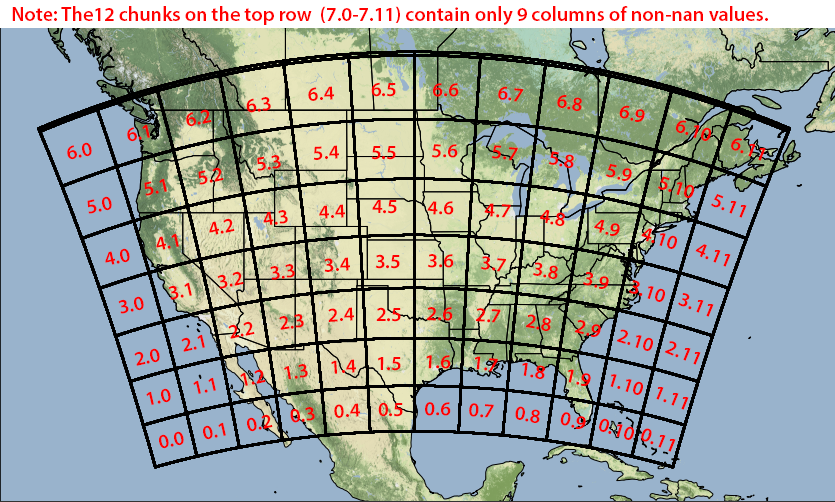
[chunk] - The conus HRRR data is broken up into 96 chunks or sections. View the map for an idea of the size and location of the chunks. The chunk identifier format differs depending on whether you have a anl or a fcst file. For fcst files the format is 0.y.x and for anl the format is y.x where the y and x are the corresponding numbers.

Python Access

We recommend three main ways of accessing the data:

• Open and decompress a single chunk
• Access the whole grid for a given hour and variable using the zarr library
• Access the whole grid for a given hour and variable with partial CF metadata using the xarray library

The following code snippets are provided for "quick start" purposes. See the rest of the code documentation for further explanation and usage.

Option 1 - Chunk Access

import s3fs
import numcodecs as ncd
import numpy as np

url = "s3://hrrrzarr/sfc/20200801/20200801_00z_anl.zarr/1000mb/TMP/1000mb/TMP/4.3"
s3 = s3fs.S3FileSystem(anon=True)

def retrieve_data(s3_url):
    with s3.open(s3_url, 'rb') as compressed_data:
        buffer = ncd.blosc.decompress(compressed_data.read())

        dtype = "<f2"
        if ("surface/PRES" in s3_url
            or "mean_sea_level/MSLMA" in s3_url
            or "0C_isotherm/PRES" in s3_url): # Pressures above 1000hPa use a larger data type
            dtype = "<f4"

        chunk = np.frombuffer(buffer, dtype=dtype)
        
        gridpoints_in_chunk = 150*150
        number_hours = len(chunk)//gridpoints_in_chunk

        if number_hours == 1: # analysis data is 2d
            data_array = np.reshape(chunk, (150, 150))
        else: # forecast data is 3d but of varying length in time
            data_array = np.reshape(chunk, (number_hours, 150, 150))

    return data_array

chunk_data = retrieve_data(url)
print(np.mean(chunk_data))

316.2

Option 2 - Zarr library

import s3fs
import zarr

url = "s3://hrrrzarr"
fs = s3fs.S3FileSystem(anon=True)
store = zarr.open(s3fs.S3Map(url, s3=fs))

temperature = store["sfc/20200801/20200801_00z_anl.zarr/1000mb/TMP/1000mb/TMP"]
index = store["grid/HRRR_chunk_index.zarr"]

import cartopy.crs as ccrs
import matplotlib.pyplot as plt

ax = plt.axes(projection=ccrs.Mercator())
ax.contourf(index["longitude"], index["latitude"], temperature, transform=ccrs.PlateCarree())
ax.coastlines()
plt.show()

Option 3 - xarray

import s3fs
import xarray as xr
import cartopy.crs as ccrs
import metpy

group_url = 's3://hrrrzarr/sfc/20200801/20200801_00z_anl.zarr/surface/GUST'
subgroup_url = f"{group_url}/surface"

fs = s3fs.S3FileSystem(anon=True)    
ds = xr.open_mfdataset([s3fs.S3Map(url, s3=fs) for url in [group_url, subgroup_url]], engine='zarr')

projection = ccrs.LambertConformal(central_longitude=262.5, 
                                   central_latitude=38.5, 
                                   standard_parallels=(38.5, 38.5),
                                    globe=ccrs.Globe(semimajor_axis=6371229,
                                                     semiminor_axis=6371229))

ds = ds.rename(projection_x_coordinate="x", projection_y_coordinate="y")
ds = ds.metpy.assign_crs(projection.to_cf())
ds = ds.metpy.assign_latitude_longitude()    
ds

<xarray.Dataset>
Dimensions:                  (x: 1799, y: 1059)
Coordinates:
  * x                        (x) float64 -2.698e+06 -2.695e+06 ... 2.696e+06
  * y                        (y) float64 -1.587e+06 -1.584e+06 ... 1.587e+06
    metpy_crs                object Projection: lambert_conformal_conic
    latitude                 (y, x) float64 21.14 21.15 21.15 ... 47.85 47.84
    longitude                (y, x) float64 -122.7 -122.7 ... -60.95 -60.92
Data variables:
    GUST                     (y, x) float16 dask.array<chunksize=(150, 150), meta=np.ndarray>
    forecast_period          timedelta64[ns] ...
    forecast_reference_time  datetime64[ns] ...
    height                   float64 ...
    pressure                 float64 ...
    time                     datetime64[ns] ...

import cartopy.crs as ccrs
import matplotlib.pyplot as plt

ax = plt.axes(projection=projection)
ax.contourf(ds.x, ds.y, ds.GUST)
ax.coastlines()
plt.show()